NEUTRALITY OF
PROFIT TAXES UNDER INFLATION AND UNCERTAINTY
by
WAYNE MAYO
This paper provides some theoretical support for material in MyProject relating to neutrality of investment decisions. It is a slightly refined version of the paper by Wayne Mayo: ‘(Tax) Depreciation and Inflation: Some Practical Observations’, Economic Papers, Vol 3, No 4, December, pp30-47, 1984.
The paper focuses on the appealing prospect of governments being able to collect tax on business profits without significantly affecting business decisions even in the presence of business risks and inflation (ie ‘neutral’ taxation). It concentrates on income taxation but also briefly considers cash flow taxes.
While much of the paper’s discussion of income taxation deals with depreciating assets, the taxation principles discussed are generally applicable to all business assets and liabilities. The paper does not analyse the distinction between direct ownership of assets and liabilities and indirect ownership via entities, such as companies or trusts. Personal and entity taxation are assumed to be fully integrated – so that annual profits at the entity level are sheeted home to individual owners in the same year.
Greater depth of discussion and analysis is available on both business income taxation and cash flow taxation in Wayne Mayo's books on these subjects: 'Taxing Investment Income - without affecting worldwide investment decisions', Kyscope Publishing, 2011'; and 'Taxing Resource Rent - concepts, misconceptions and practical design', Kyscope Publishing, 2013.
- Introduction
- Neutral Profit Taxes Under Certainty
- Tax With Interest Excluded (Cash Flow Taxation)
- Tax With Nominal Interest Included (Taxation of Nominal Income)
- Related Issues
- Conclusions
- Appendix1: General Discounting Principle
- Appendix 2: Rate of Decline of Net Receipts
- Appendix 3: Effect of Depreciation Allowances Applied to Asset Cost when NPV>0
- References
- Neutral Profit Taxes Under Certainty
INTRODUCTION
‘Neutral’ taxation of business profits (profits
from investment activity) would leave before-tax investment decisions
unaffected. This paper aims to
demonstrate, using simple discounting concepts, two separate sets of requirements
for neutrality of profit taxes regardless of the level of inflation (but,
initially, in the absence of risk):
· immediate write-off of capital expenditure with the exclusion of interest from the tax base, which forms the conceptual basis of cash flow taxes generally and, in particular, the resource rent tax scheme applying to petroleum projects in ‘green fields’ offshore areas in Australia; or
· the allowance of economic depreciation (or actual change in asset
value) with the inclusion of nominal interest in the tax base, which forms
the conceptual basis of Australia's business income tax system. Income taxation is the main focus of the
paper.
The
achievement of income tax neutrality in practice is often all too readily
dismissed because economic depreciation is thought to be unattainable. The analysis here shows, however, that with
constantly-deteriorating depreciating assets economic depreciation can,
regardless of the level of inflation, be estimated in practice using as a basis
the reducing balance method of determining depreciation allowances. While the practical application of economic
depreciation concentrates on investment in depreciating assets, the taxation
principles involved are applicable to other assets, liabilities and investment
projects generally.
The paper also uses simple discounting concepts to show that the taxation allowances required for neutrality when real interest is incorporated in the tax base comprise economic depreciation plus additional year-by-year deductions reflecting the annual loss in real value from inflation.
Finally,
risk is introduced to show how the results of the analysis under certainty are
generally applicable to the more realistic situation of investment uncertainty.
Neutral Profit Taxes Under Certainty
To
highlight the tax-related issues, take a situation where there is a known
current and future 8% rate of inflation for prices generally and a healthy
capital market enabling people to borrow or lend as much as they like at the
going inflation-affected nominal 15% interest rate. The future net revenue stream from any capital investment is also
known with certainty and there is always sufficient income to write off tax
deductions in full in the year they become available (that is, ‘full loss
offset’ applies). Personal and company
taxation are fully integrated.
Exactly how, or to what extent, the nominal interest rate has adjusted to inflation is not important. The analysis focuses on the neutrality of investment decisions after tax and with inflation, compared to the pre-tax situation under the same inflationary conditions (with the going interest rate unaffected by the tax).
Before tax,
marginal capital investments are those with returns just equal to the going 15
% interest rate, or with a net present value (NPV) of zero with discounting at
that interest rate. The return from
those investments just compensates entrepreneurs for the opportunity cost of
tying up their money in them. One such
marginal before-tax investment can be represented, with discounting at the 15%
rate, by:
NPVb = R – C = 0 (1)
where NPVb = net present value of the investment before tax;
R = value of discounted end-of-year
receipts including any asset
sale value, less operating expenses;
and
C = price of asset at the start of the
first year.
Any loan
funding used to purchase the asset need not be included explicitly as the
equity contribution plus the present value (PV) of the repayments of any loan
is the price of the asset.
After tax,
we want these same investments to remain marginal. In other words, we want the capital allowances for tax purposes
to be such that these investments provide the entrepreneur with the same after-tax
return that could be obtained from putting the investment funds in the cash
market. That is, with discounting at
each entrepreneur's after-tax opportunity cost of money, the NPV of these
investments should remain zero.
Tax With Interest Excluded (Cash Flow Taxation)
A tax with interest excluded does not affect entrepreneurs' before-tax discount rate. They are still able to receive their 15% from the financial market after the tax.
In these circumstances, allowing immediate write-off of capital expenditure (and including any sale value in assessable income) results in the initial investment outlay, as well as the net receipts in each year, being reduced by a proportion equal to the tax rate applicable to the entrepreneur. Thus, the tax-reduced net receipts and sale value represented in equation (1), discounted at the same 15%, equal the price of the asset reduced by the effect of writing off this capital cost immediately against other income. The investment remains marginal after tax.
More
generally, the relationship between the NPV of an investment before and after
this cash flow – or Brown (1948)
– tax, as shown by Mayo (1979)
using these simple discounting observations, is given by:
NPVa = (R - C) (1 - t) = NPVb(1
- t) (2)
where t = the entrepreneur's marginal tax rate.
If NPVb
is zero (marginal) before tax, it remains zero (marginal) after tax. This neutrality condition holds regardless
of the rate of inflation or the particular marginal tax rate of the
entrepreneur.
Because the
before-tax discount rate is not directly affected by the cash flow tax, the tax
is well suited as an additional tax or royalty on a particular sector of an
economy. A resource rent tax (RRT) is a
variant of this cash flow tax with losses being carried forward at a specified
‘threshold’ rate when, in practice, sufficient other income is not available to
offset fully available deductions in the year they arise. Under our assumption of certainty, this
‘threshold’ rate would equal the going nominal interest rate if the RRT is
imposed before income tax. When the
losses carried forward at this rate are eventually recouped, their value as a
tax deduction in discounted terms will be equal to that value had full loss
offset been available. (Uncertainty is
introduced in the later section on risk.)
Tax With Nominal Interest
Included (Taxation of Nominal Taxation)
In contrast
to the cash flow tax, an income tax with nominal interest included in the tax
base does affect entrepreneurs' before-tax discount rate. If an entrepreneur faces a 46% income tax
rate, the 15% before-tax return from the financial market will be reduced in
proportion to this tax rate to 8.1%.
Nevertheless,
with economic depreciation allowed and with discounting at 8.1%, the investment
represented by equation (1) will still have a NPV of zero. The entrepreneur will, after tax, still be
indifferent between receiving 8.1% from the financial market and 8.1% from that
capital investment. This comes about
because both C and R in equation (1) remain the same as they were before tax
with discounting at 15%.
Appendix 1
uses a general discounting principle to show that the cost of the asset, C, is
unaffected regardless of the level of debt used to acquire it. This is because the before-tax discount rate
(the going interest rate) and the interest component of any loan repayments are
reduced by the tax in proportion to the entrepreneur's tax rate. In these circumstances, the after-tax PV of
any loan repayments is again the initial value of the loan. Thus, after the income tax, the equity
contributions and the PV of the stream of any net loan repayments still sum to
the price of the asset.
Similarly,
Appendix 1 shows that for the net receipts stream represented in equation (1)
to discount after tax to R, only the ‘interest component’ of the before-tax net
receipts in each year must be reduced by a proportion equal to the
entrepreneur's tax rate. That is, the
‘principal component’ of the net receipts in each year must be an allowable
deduction for income tax purposes, so that only the ‘interest component’ is
taxed. With net receipts obtaining at
the end of each year, the ‘principal component’ of the net receipts in any year
is the difference in the PV of the net receipts stream at the start and end of
that year, or the difference in the value, including the inflationary
component, of the asset over that year. That difference is economic depreciation.
As shown by Samuelson (1964) and others since, such as Swan (1976), this neutrality of a nominal income tax system allowing economic depreciation applies regardless of the rate of inflation and of the marginal tax rate of the particular entrepreneur who is deciding the viability of an investment. In contrast to the cash flow tax, the neutrality of the income tax depends on its direct effect on entrepreneurs' after-tax discount rates, an effect which can only be achieved if the tax is applied economy-wide and not to just one particular sector.
Economic
Depreciation in Practice with Depreciating Assets
It is often
assumed that economic depreciation cannot readily be determined in practice for
depreciating assets and allowed for income tax purposes. Most income tax systems, including
Australia’s, however, provide for a balancing adjustment on the disposal of
depreciable assets. That disposal
adjustment ensures that, over the years of use of a depreciating asset by one
owner, only the difference between the asset’s original cost and its final sale
value is allowed for tax purposes (except to the extent that any nominal
capital gain realised is not taxed).
Thus, economic depreciation is usually already allowed over the time
that a depreciating asset is owned by a taxpayer. The depreciation provisions for tax purposes really specify the
structure of write-off of change in economic value year by year over the period
that a taxpayer owns a depreciating asset.
Further,
for a marginal asset physically deteriorating at a constant rate (more
generally, value declining at a constant rate with no inflation), economic
depreciation is changing year by year by the same proportion as its net
receipts are changing (Appendix 2).
With deterioration at the rate s and inflation at the rate i, the
asset's net receipts, say P, in one year change to (1 – s)(l + i)P the next, so
its net receipts and economic value change each year by the proportion (1 –
s)(l + i) - 1.
Therefore,
if K is the depreciated value (or, in modern parlance, ‘tax value’) of the
asset at the start of a year, economic depreciation, D, for that year (defined
positive here if the proportional change in economic value is negative) is
given by:
D = (1 - (1 – s)(l + i))K
= (s(l + i) - i)K
= sK - i(1 - s)K (3)
This
result, illustrated in Table 1, is equivalent to that obtained by King (1977,
p. 242) for his debt financing case and corresponds to Proposition 1A of Swan
(1978, p. 3).
With no
inflation, equation (3) shows that the annual economic depreciation of a
marginal asset, sK, corresponds to the income tax allowance obtained from the
standard declining balance method applied to historical cost at the rate of
physical deterioration (or, more generally, at the constant rate of decline in
value in the absence of inflation).
Under the Australian ‘effective life’ depreciation arrangements, the
Commissioner of Taxation determines the effective lives of categories of
depreciable assets. The effective lives
translate into reducing balance depreciation rates 1.5 times the alternative
straight line rate. Consequently, under
non-inflationary conditions, if the declining balance rate determined under
this system corresponds to the constant rate of decline in value of that type
of asset, the reducing balance allowances based on historical cost would equate
with economic depreciation.
Under
inflationary conditions, however, equation (3) shows that such ‘standard’
historical cost allowances for capital assets (and stocks) would be too
generous. In practice, from the
allowance in a particular year, determined by applying the declining balance
rate to the depreciated value at the start of the year, would be subtracted an amount
equal to the proportion i(l - s) of that same depreciated value. The economic depreciation so obtained would
determine the asset's depreciated value at the start of the next year, and so
on until the asset was scrapped or sold.
With
inflation, the depreciated value under reducing balance write-off would, in the
early years, fall year by year further and further below the true economic
value of the asset. Eventually, in
later years the depreciated value would become so low that the annual depreciation
allowances from the reducing balance method would become less than the actual
economic depreciation in those years.
Once the asset was sold, however, the balancing adjustment on disposal
would generally ensure that the sum of the income tax allowances equalled the
economic depreciation of the asset over its period of use. This is illustrated in Table 1.
TABLE
1: EFFECT OF INFLATION ON ASSETS WITH DIFFERENT RATES
OF PHYSICAL DETERIORATION UNDER AN INCOME TAX INCORPORATING NOMINAL INTEREST
(a)
|
Year |
Invest-ment |
Net Rec’pts |
Economic Depreci-ation (b) |
DB(Hist. Cost) Dep’n (c) |
Tax Econ Dep’n |
Tax DB |
Cash Flow Econ
Dep’n |
Cash Flow DB |
Long-lived Asset (s = 0.15)
|
0 |
1000.0 |
|
|
|
|
|
-1000.0 |
-1000.0 |
||||
|
1 |
|
232.0 |
82.0 |
150.0 |
69.0 |
37.7 |
163.0 |
194.3 |
||||
|
2 |
|
213.0 |
75.3 |
127.5 |
63.3 |
39.3 |
149.6 |
173.7 |
||||
|
3 |
|
195.5 |
69.1 |
108.4 |
58.1 |
40.1 |
137.4 |
155.4 |
||||
|
4 |
|
179.5 |
63.4 |
92.1 |
53.4 |
40.2 |
126.1 |
139.3 |
||||
|
5 |
-651.9 |
164.8 |
58.2(e) |
-129.9(f) |
49.0 |
135.6 |
767.7 |
681.1 |
||||
|
PV at 15%
0.0 |
|
|
236.3 |
221.5 |
0.0 |
14.8 |
||||||
|
Effective Tax Rate (g) |
|
|
|
|
46.0% |
43.1% |
||||||
Short-lived Asset (s=0.375)
|
0 |
1000.0 |
|
|
|
|
|
-1000.0 |
-1000.0 |
||||||
|
1 |
|
475.0 |
325.0 |
375.0 |
69.0 |
46.0 |
406.0 |
429.0 |
||||||
|
2 |
|
320.6 |
219.4 |
234.4 |
46.6 |
39.7 |
274.1 |
281.0 |
||||||
|
3 |
|
216.4 |
148.1 |
146.5 |
31.4 |
32.2 |
185.0 |
184.2 |
||||||
|
4 |
|
146.1 |
100.0 |
91.6 |
21.2 |
25.1 |
124.9 |
121.0 |
||||||
|
5 |
-140.0 |
98.6 |
67.5(e) |
12.5(f) |
14.3 |
39.6 |
224.4 |
199.1 |
||||||
|
PV at 15%
0.0 |
|
|
153.8 |
147.2 |
0.0 |
6.6 |
||||||||
|
Effective Tax Rate (g) |
|
|
|
|
46.0% |
44.0% |
||||||||
- Inflation, i, is at 8%, the nominal interest rate at 15% and tax at 46%. The NPV before tax of both investments is zero. With no inflation, the long-lived asset's net return in period 1 would be $214.8 reducing by 15% per year, and the short-lived asset's net return would be $439.8 reducing by 37.5% per year.
- To the depreciated value (asset cost less
allowed economic depreciation) at the end of the previous year, the rate of
deterioration, s, is applied less the inflationary adjustment i(1 – s). This is the practical estimation of annual
economic depreciation.
- Declining balance depreciation at the rate of physical decline, s, of the asset (including balancing adjustment on disposal in period 5).
- With discounting at the after-tax rate of 8.1
%, the NPV is again zero (and the effective tax rate 46%).
- Balancing adjustment on disposal is $0.0.
- Balancing adjustment on disposal is $208.2 and
$44.8 for the long- and short-lived asset respectively.
- With economic depreciation or reducing balance depreciation applied at the asset's rate of physical deterioration, the effective tax rate may alternatively be determined by dividing the PV of the actual tax payments by the PV of the taxable income were economic depreciation allowed. (This PV method could incidentally, be a more generally appropriate way of defining effective tax rates.)
Because the
historical cost reducing balance allowances must be greater than economic
depreciation in the early years, the PV of the historical cost allowances will
be greater than the PV of economic depreciation allowances. During periods of inflation, depreciation
allowances based on historical cost (under implied non-inflationary conditions)
are ‘accelerated’ compared to the neutral case, as shown in Table 1. As Swan (1978, p. 7) points out, the ‘tax
liability of the firm is reduced in the relevant present value sense by the
impact of inflation which drives a wedge between economic and historical based
depreciation schemes’. Thus, statutory
accelerated depreciation provisions such as, at the extreme, 100% write-off in
the year of expenditure in no way counteract the effects of inflation on
historical cost depreciation allowances.
They actually exacerbate the generosity of the historical cost allowances.
The
acceleration of the historical cost allowances could be removed in practice by
determining appropriate effective lives or rates of value decline of constantly
deteriorating asset types (under implied zero inflation) and applying equation
(3) as described above. Depreciation
allowances would be an estimate of annual economic depreciation. Of course, all assets would not be expected
to have a neat constant rate of deterioration.
Nevertheless, studies by Hulten and Wykoff (1981) have suggested that
the physical deterioration profile of many types of assets does indeed
approximate that of a constantly deteriorating asset. To the extent that an asset tended towards either linear
depreciation or the ‘one-horse-shay’ type, with net receipts maintained at the
same level until there is total collapse, equation (3) would still generally
provide year-by-year allowances which were too generous. With a marginal ‘one-horse-shay’ asset, for
example, economic depreciation actually increases during the life of the asset
and corresponds to the principal components of a loan at the going interest
rate over the life of the asset with repayments equal to the constant annual
net receipts.
The result
that, with inflation, historical cost allowances are too generous may seem
counter-intuitive. But the result takes
into account considerations sometimes ignored: the effect of inflation on the
year-by-year nominal value of the asset; and the fact that the full nominal
value, and not just the real value, of interest payments is included in the tax
base. As Appendix 1 shows, taking into
account the effect on the entrepreneur's discount rate, a nominal income tax
system incorporating economic depreciation maintains before-tax nominal wealth
(value of marginal assets) regardless of the investment undertaken. The entrepreneur's real wealth (command over
future real consumption) may be affected, but it will be affected in the same
way for both the capital investment and the alternative financial investment to
maintain the balance between these two alternatives. This balance would, however, be upset by providing the capital
investment accelerated depreciation: with nominal interest income being taxed
in full, nominal income from capital investments is also required to be taxed
in full to achieve neutrality.
Effective Tax Rates
‘Effective
tax rate’ is defined as the difference in the before and after-tax nominal
rates of return expressed as a percentage of the before-tax nominal rate of
return. The neutrality condition of zero
NPV before and after income tax is therefore the same as requiring the
effective tax rate to be equal to the statutory tax rate. This equivalence results directly from the
fact that the entrepreneur's before-tax discount rate is reduced by the tax by
a proportion equal to the relevant marginal tax rate. Thus, the effective tax rates in Table 1 equal the statutory rate
when economic depreciation is allowed, and are less than the statutory rate
with historical cost depreciation allowed.
In general
terms, effective tax rates compare actual tax payments, according to the system
under study, with the taxable income that would be applicable under the neutral
tax system which incorporates interest in the same way – either nominal, real, or excluded completely – as the system under study. In terms of investment neutrality, it would
be meaningless to compare, say, the actual income tax paid under a system which
has nominal interest included, with taxable income under a neutral tax system
which incorporated real interest.
The
Choice of Asset Lives and Repairs versus Replacement
As shown
from equation (3), the closer the rate of physical decay to unity (or the
shorter the life of the asset), the closer will be the PV of the historical
cost declining balance allowances plus disposal adjustment to the PV of
year-by-year economic depreciation.
Consequently, the shorter the life of an asset marginal before tax, the
closer will the (positive) after-tax NPV of the asset be to zero.
Thus, in
times of inflation, with an income tax system incorporating nominal interest
and historical cost depreciation allowances, investment decisions will be
biased towards assets with longer-lives.
This bias is illustrated in Table 1 where the NPVs of the shorter- and
longer-lived assets are $6.6 and $14.8 respectively, which
correspond to effective tax rates of 44.0% and 43.1%.
Similarly,
during periods of inflation, decisions would be biased away from year-by-year
repairs to existing plant with associated year-by-year deductions and towards
‘longer-lived’ expenditure on replacement or capital modification of existing
plant with associated deductions for depreciation over the effective life of
the capital investment. Further, because
the balancing adjustment on disposal brings back to assessment at the time of
sale reducing balance deductions allowed over the period of asset use in excess
of economic depreciation, historical cost allowances under inflation would tend
to distort decisions towards longer asset holding.
The
generosity of statutory write-off arrangements, such as write-off in the year
of expenditure, bias decisions towards longer-lived assets even when there is
no inflation, and the generosity of these arrangements is magnified during
periods of inflation. With write-off in
the year of expenditure, for example, the effective tax rates faced by the two
investments in Table 1 would be 26.7% and 19.6% for the shorter- and
longer-lived asset respectively.
The
reductions in effective rates in the above illustrations do not imply that,
despite the distortions imposed, everyone would gain from the introduction of
generally available first-year write-off of capital expenditure. With everyone receiving the same generous
treatment, there would be consequential offsetting general adjustments in terms
of, for example, prices, interest rates, and exchange rates, and all that would
remain after these had worked their way through the economy would be the
distortions around the new ‘margin’ (and, of course, the transitional revenue
losses associated with the introduction of accelerated depreciation). To the extent that any, perhaps relatively
capital intensive, firm or industry benefited it would be at the expense of
others; everyone would, in effect, be worse off. Any potential macroeconomic stimulation aimed at could be better
achieved by less distortive measures.
RELATED ISSUES
Tax With Real Interest
Included (Taxation of Real Income)
After
imposing an economy-wide income tax incorporating symmetrical treatment of real
interest payments and receipts, only the real part of the entrepreneur's 15%
return from the financial market would be taxed at the 46% rate. With 8% inflation, only the real 7% would be
taxed, reducing the 15% return by 3.22% to 11.78%.
Looked at
another way, the nominal 15% return would be taxed in full, leaving the 8.1%
return as in the nominal interest case, and a refund of tax provided for the
excess 3.68% tax paid on the 8% inflationary component. Thus, the entrepreneur's discount rate would
be increased, compared with that in the nominal interest case, by a factor
equal to the tax rate times the inflation rate. Symmetrically, the entrepreneur would be allowed deductibility of
real interest payments, which is the same as being allowed a deduction in full
of nominal interest payments (as in the nominal interest case) and in addition
being taxed on the fall in the real value of net monetary liabilities in each
year.
As shown in
Appendix 1, these effects on loan repayments and on the discount rate mean
that, again, C in equation (1) is unaffected by this tax regardless of the
gearing ratio used to acquire the asset.
Similarly, for the revenue stream of the asset to discount (at each
entrepreneur's after-tax discount rate) after tax to R in equation (1), thus
keeping the investment marginal after tax, taxation allowances are required in
addition to economic depreciation allowances.
Appendix 1 shows that this additional allowance in each year is the
inflation rate times the PV of the asset's revenue stream at the start of the
corresponding year (i.e. the value of the asset at that time or, in practical
terms, the depreciated value of the asset when economic depreciation is
allowed). That is, for constantly deteriorating
assets, the taxation allowances needed to achieve neutrality are given by:
A = (s(1 + i) - i)K + iK (4)
The
additional capital allowance, iK, is the asset's annual loss in real
value. This result, illustrated in
Table 2, is that derived by King (1977, p. 242), again for his debt financing
case, and is equivalent to Proposition 2A of Swan (1978, p. 4).
These
arrangements not only maintain the entrepreneur's nominal wealth but, as Swan
(1982) points out, they also maintain before-tax real wealth, thus avoiding any
inequities resulting from real wealth effects of the nominal interest
system. This real interest system may
also better hold up against the assumption of an unchanged nominal interest
rate with the imposition of tax.
TABLE
2: EFFECT OF INFLATION ON ASSETS WITH DIFFERENT RATES
OF PHYSICAL DETERIORATION UNDER AN INCOME TAX INCORPORATING REAL INTEREST (a)
|
Year |
Invest-ment |
Net Rec’pts |
Economic Depreci-ation (b) |
Additional allowance (c) |
Tax Econ Dep’n |
Tax 1 year (d) |
Cash Flow Econ Dep’n
(e) |
Cash Flow 1
year (d) |
Long-lived Asset (s = 0.15)
|
0 |
1000.0 |
|
|
|
|
|
-1000.0 |
-1000.0 |
||||||
|
1 |
|
232.0 |
82.0 |
80.0 |
32.2 |
-353.3 |
199.8 |
585.3 |
||||||
|
2 |
|
213.0 |
75.3 |
73.4 |
29.6 |
98.0 |
183.4 |
115.0 |
||||||
|
3 |
|
195.5 |
69.1 |
67.4 |
27.1 |
89.9 |
168.4 |
105.6 |
||||||
|
4 |
|
179.5 |
63.4 |
61.9 |
24.9 |
82.6 |
154.6 |
96.9 |
||||||
|
5 |
-651.9 |
164.8 |
58.2(f) |
56.8 |
22.9 |
375.7(g) |
793.8 |
441.0 |
||||||
|
PV at 15%
0.0 |
|
|
101.0 |
94.9 |
0.0 |
6.0 |
||||||||
|
Effective Tax Rate (h) |
|
|
|
|
46.0% |
41.8% |
||||||||
Short-lived Asset (s=0.375)
|
0 |
1000.0 |
|
|
|
|
|
-1000.0 |
-1000.0 |
||||||
|
1 |
|
475.0 |
325.0 |
80.0 |
32.2 |
-241.5 |
442.8 |
716.5 |
||||||
|
2 |
|
320.6 |
219.4 |
54.0 |
21.7 |
147.5 |
298.9 |
173.1 |
||||||
|
3 |
|
216.4 |
148.1 |
36.5 |
14.7 |
99.6 |
201.8 |
116.9 |
||||||
|
4 |
|
146.1 |
100.0 |
24.6 |
9.9 |
67.2 |
136.2 |
78.9 |
||||||
|
5 |
-140.0 |
98.6 |
67.5(f) |
16.6 |
6.7 |
109.8(g) |
232.1 |
128.9 |
||||||
|
PV at 15%
0.0 |
|
|
66.9 |
79.2 |
0.0 |
-12.4 |
||||||||
|
Effective Tax Rate (h) |
|
|
|
|
46.0% |
57.2% |
||||||||
- The NPV before tax of both investments is zero as in Table 1.
- As in Table 1.
- Depreciated value at the end of the previous period times the rate of inflation, 8%.
- Tax payments with write-off in the year of
expenditure allowed.
- With discounting at the after-tax rate of
11.78%, the NPV is again zero (and the effective tax rate 46%).
- Balancing adjustment on disposal is $0.0.
- Includes balancing adjustment on disposal of $651.9 and $140.0 for the long- and short-lived assets respectively.
- Effective tax rates in the real interest case are determined by expressing the difference between the real before- and after-tax rates of return as a percentage of the real before-tax return. Regardless of the levels of inflation and the nominal interest rate, the real before-tax interest rate, reduced by the tax rate proportion, equals the real after-tax rate. Thus, with the neutral taxation allowances, the effective tax rate equals the nominal tax rate.
With the
constant rate of 8% inflation assumed here for both capital goods and prices
generally, the taxation allowances in equation (4) reduce to s(1 + i)K. This formulation can be somewhat misleading
from a practical viewpoint. The
taxation allowances required for neutrality are best viewed as comprising two
quite distinct components: economic depreciation allowances, which could be
determined in practice according to equation (3) on the assumption of
constantly deteriorating assets; and an additional capital allowance, which
would depend on the general rate of price increases used to determine the real
component of interest payments and receipts for income tax purposes. The important point here is that the
additional capital allowance would not be part of the depreciation allowances
for income tax purposes: it would not be used in determining the depreciated
value of the asset at any time, and it would not come into the determination of
the balancing adjustment for taxation purposes when the asset is sold. The effect of the additional capital
allowance is to maintain the indifference of the entrepreneur between investing
in an asset which is marginal before tax and investing in the financial market
when only the real component of interest from his financial investment is
taxable.
The reduced
form of equation (4) shows, however, that with uniform inflation, standard
historical cost reducing balance allowances set on the basis of zero inflation
would be less generous than the combination of economic depreciation and the
deductibility of the loss in real value, and would result in effective tax
rates greater than the nominal tax rate.
Accelerated depreciation allowances may, for particular types of assets,
be more appropriate than the historical cost allowances. Write-off allowed in the year of
expenditure, for example, reduces the effective tax rates of the short-lived
and long-lived assets illustrated in Table 2 below the rates applicable with
historical cost depreciation, to 57.2% and 41.8% respectively. An asset with a life somewhat shorter than
the long-lived asset would, with first year write-off, just attract an
effective tax rate of 46%, the same rate that would apply were economic
depreciation allowed plus the loss in real value.
Thus, it is
with real (and not nominal) interest incorporated in the system that particular
statutory accelerated depreciation allowances, substituting for the allowances
in equation (4), may at least adjust in the right direction for the effect of
inflation. But a statutory adjustment
would only be appropriate at a specific level of inflation and for assets with
a specific rate of physical deterioration.
Relative biases between assets with different lives would be
unavoidable.
Risk
With
certainty in relation to the net receipts stream, the investment ‘margin’
corresponds to the going return from the financial market. When net receipts streams are not known with
certainty, the investment margin of a particular entrepreneur can be imagined
as a continuum of NPV probability distributions corresponding to marginal
capital investments of different levels of risk. At one extreme in this continuum is the riskless investment, with
a sure zero NPV and a before-tax return corresponding to the going rate of
interest. As the spread of possible
outcomes of investments in this continuum increases, the expected NPV also
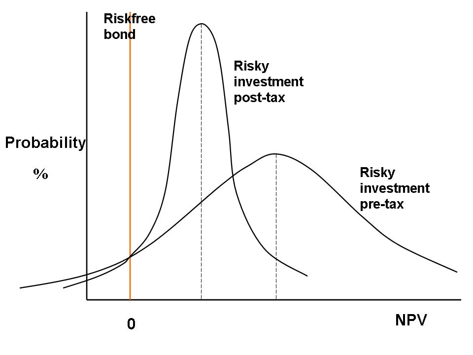
increases to balance the increased risk (Figure 1).
Each risky
capital investment in this continuum would be judged marginal by the
entrepreneur. Ideally, the entrepreneur
would establish its NPV probability distribution by obtaining the NPV for each
possible net receipts stream from that investment at his riskfree discount rate
(before tax, the going interest rate).
This probability distribution would contain all the information about
risk. To use a risk-weighted discount
rate to build up the distribution would be double counting.
In broad
terms, a tax would be neutral under uncertainty if it had a symmetrical impact
on the loss-making end and the profitable end of the range of possible outcomes
of each capital investment on the entrepreneur's before-tax continuum of marginal
distributions, such that the investment remained on that continuum after
tax. This symmetrical impact would
result with the neutral cash flow tax from its proportional effect –
equation (2) – on before-tax positive NPVs and, assuming full loss offset (the
ability to write off annual losses against other income immediately), negative
NPVs (Figure 1).
With the income
taxes incorporating economic depreciation, the relationship of equation (1)
is maintained after tax with riskfree investments. It is also maintained with any of the many possible outcomes of a
risky investment that happen to produce a zero NPV before tax (that is, with a
return equal to the going interest rate).
But the relationship of equation (1) is not maintained with possible
outcomes of a risky investment which have a positive or negative NPV before
tax. These positive or negative NPVs
arise because the asset's market price (at the time of purchase or later)
differs from its value from the entrepreneur’s point of view, as reflected in
its future receipts stream discounted by the entrepreneur at the going interest
rate. The greater the difference
between price and value to the entrepreneur the greater is the absolute value
of the NPV. If that difference were
included in the entrepreneur’s income tax base, the NPV would again be reduced
in proportion to the entrepreneur’s tax rate, consistent with equation (2) and
Figure 1 (again assuming full loss offset).
In
practice, of course, it would be impracticable to measure differences between
price and value to the entrepreneur and include these differences in his tax
base. A depreciating asset's price, for
example, has to be taken as its economic value at the time of purchase and used
as the basis for annual depreciation allowances. Thus, for possible investment outcomes with non-zero NPVs, even
if the physical deterioration of the associated depreciating assets were at a
constant rate, the year-by year economic depreciation for them would not be
given by equations (3) and (4). These
equations only apply to investments with prices reflecting their future net
receipts streams. To illustrate the
implications of this, Appendix 3 analyses the effect on possible investment
outcomes with NPVs greater than zero of applying depreciation allowances from
equation (3) to asset cost rather than value in the nominal interest case.
FIGURE 1: RISKFREE BOND AND MARGINAL RISKY INVESTMENT PRE- AND POST-CASH FLOW TAX
Appendix 3
points to proportional reductions in positive NPVs of possible investment
outcomes across constantly deteriorating assets, with those proportional
reductions independent of asset cost, net receipts and residual values.
Thus, with constantly deteriorating assets, the use of equations (3) or
(4) would still mean that the respective ‘neutral’ income taxes would have a
symmetrical impact on the NPV probability distribution of prospective
investments.
In sum, for
investments generally, the theoretical inclusion in the income tax base of the
difference between market price and value of assets to the investor would have
a ‘squeezing’ effect the NPV probability distributions around the zero NPV
outcome, like that in Figure 1. And in
the case of depreciating assets, at least, practical estimates of annual
economic depreciation would have similar effects on after income tax NPV
probability distributions.
Thus, the
effect of the cash flow and income taxes neutral under uncertainty would, in
broad terms, be to ‘squeeze’ each NPV probability distribution in an
entrepreneur's continuum of marginal distributions proportionately closer to
the riskless investment earning a sure return equal to the entrepreneur's
after-tax discount rate. While
risk-averse entrepreneurs would usually be expected to require a greater than
proportional decrease in the expected NPV of an investment to balance a
proportional decrease in the associated risk, the effect of the neutral taxes
would broadly be to keep investments which were on an entrepreneur's marginal
continuum before tax on his continuum after tax. The taxes would, in broad terms, be neutral under uncertainty.
The
proportional effect on the loss-making end of the NPV probability
distributions, or a symmetrical ‘squeeze’, requires full loss offset to
apply. In the absence of full loss
offset, maintaining the value of any annual losses carried forward under either
cash flow or income taxes theoretically requires those losses to be carried
forward with an interest or threshold rate added to maintain their value as a
deduction. As noted earlier, with no
risk the threshold rate would be the going interest rate. Under uncertainty, the threshold rate for
such loss carry-forward would still be the going rate of a riskless investment
but only if it were certain that the compounded losses would ultimately be
deducted. To the extent that it is
certain that any excess deductions in a particular year would be eventually
written off in full, the threshold rate required to maintain the value of the
deductions would correspond to the year-by-year cost of having to wait to
recoup that certain value.
Thus, even
with uncertainty, were full loss offset available (immediately or delayed),
with an RRT applied before income tax the appropriate threshold rate would
correspond to, say, the going long term bond rate. When write-off provisions do not completely remove the risk of
undeducted losses, the NPV probability distribution of a potential project may
be skewed by the neutral taxes, including an RRT. The loss-making end of the range of possible outcomes is not reduced
to balance the reduction in the profitable outcomes. It is in these circumstances, for example, that
loading the RRT threshold rate might be looked to as a method of offsetting, in
a very rough way, the effect of skewed probability distributions.
CONCLUSIONS
The main
observations in the paper can be summarised as follows:
- It is possible to design cash flow taxes or income taxes aimed at achieving neutrality of investment decisions in the presence of inflation and uncertainty. Cash flow taxes are suited to industry- or sector-specific taxation but income taxes need to apply on a national basis to achieve the required effect on after tax discount rates.
- With an income tax system such as Australia's, incorporating nominal interest in its base, economic depreciation – that is, the annual change in capital value – would offer the prospect of raising revenue with minimal impact on before-tax investment decisions. This conclusion applies generally to all business assets and liabilities, not just depreciating assets.
- With depreciating assets,
soundly based historical cost reducing balance depreciation allowances for
income tax purposes estimated on the implied assumption of zero inflation
(or associated straight line depreciation allowances) are too generous
under inflationary conditions.
These allowances bias investment decisions towards
longer-lived assets, and away from repairs and maintenance to replacement
expenditure, and encourage longer asset holding.
- For depreciating assets, these biases could largely be
removed in practice by estimating economic
depreciation by applying reducing balance rates (set according to
‘effective’ lives under implied zero inflation) together with an
adjustment based on both the inflation rate and the reducing balance
rate. Nevertheless, unavoidable
'bluntness' of across-the-board effective lives means that effective life
write-off without any additional adjustments represents a practicable
arrangement, particularly in times of relatively low inflation. As usual, differences between
depreciation write-off allowed and actual change in value are picked up by
the balancing adjustment on disposal.
- With real interest incorporated
in the income tax base, neutrality requires a tax base comprising
estimated annual economic depreciation plus annual loss in real value.
- These observations concerning
the neutrality of profit taxes under inflation are largely unaffected by
uncertainty concerning the future net receipt streams of capital
investments. The lack of sufficient
other income to immediately write-off annual losses, however, represents a
source of non-neutrality. In
practice, that non-neutrality could be addressed for both cash flow and
income taxes by carrying forward losses at a ‘threshold rate’. To the extent that the tax system
offers certainty that the compounded loss will ultimately be written off
against other income, the threshold rate would be in line with the long
term bond rate.
APPENDIX 1
General Discounting Principle
Any given
stream of numbers (with the number in each period in the stream obtaining at
the end of that period) will discount at a given discount rate, say, p, to a
specific value, say, C. In this
discounting process, the numbers can be regarded as having a principal and
interest component, as would the per period repayments of a reducing balance
loan having a value of C and interest rate p.
The
principal component of the number in each period is the difference between the
PV of the stream of numbers (value of the loan) at the start and end of the
corresponding period. The interest
component makes up the rest of the number and is equal to p times the PV of the
stream of numbers (value of the loan) to the start of the corresponding period. These definitions of principal and interest
components derive from the relationship between the PV of a stream of numbers
at the start and end of one period (say period 1):
PV1 = PV0 +
p.PV0 – N1 (4)
where PV0 = present value
at start of period 1
PV1 = present value at end of period 1
N1 = number obtaining at end of period 1
In words,
equation (4) says to get the (present) value at the end of period 1, take the
(present) value at the start of the period and:
- add an amount equal to the
discount (interest) rate times that opening value (ie the interest income
earned on the opening value over the period); and
- subtract an amount equal to the
number at the end of the period (that number drops out of the value
calculation to the start of period 2, or end of period 1).
Rearranging
equation (4),
N1 = (PV0 - PV1)
+ p.PV0 (5)
where PV0 - PV1
= principal component of N1
p.PV0
= interest component of N1
Take the
two numbers N1 and N2 (e.g. loan repayments) obtaining at
the end of two consecutive time periods.
With discounting at the rate p, the PV of the two numbers (value of the
loan) at the start of period 1 is given by:
PV0 = N1/(1 + p)
+ N2/(l + p)2 (6)
Further,
take any two proportions, t (later to represent the investor’s tax rate) and x
(later to represent minus the going interest rate in the nominal interest case
and the inflation rate in the real interest case). Add to N1 an
amount equal to x.t times the PV of N1 and N2 (value of
the loan) at the start of period 1 (with discounting at the rate p). And add to N2 an amount equal to
x.t times the PV of N2 (value of loan) at the start of period 2
(with discounting at the rate p).
Now, by
applying equation (6), the PV (value of the loan under new conditions) at the
start of period 1 of N1 and N2 plus the amounts added
to N1 and N2 with
discounting at the rate p + xt is given by:
PV0 = (1 + p)N1
+ xtN1
(1 + p)(1 + p + xt)
+ xtN2 +
(1 + p)N2
+ xtN2
(1 + p)2(1 + p + xt) (1 + p)(1 + p + xt)2
= N1/(1 + p) + N2/(l +
p)2 (7)
PV0 (value of the loan) at the start of period 1 in equation
(7) – that is, after the factor, x.t, is added to both the discount rate and,
in each period, the same factor times the value of the loan at the start the
period is added to the loan repayments at the end of the period – is the same
as PV0 in equation (6) before the changes are made to the discount
rate, p, and the two numbers N1 and N2
(loan repayments). By increasing the number of numbers and time
periods and applying the above methodology, it can be shown by induction that
this result holds for any stream of numbers.
By
selecting applicable proportions for p, t and x, and by transferring the above
references concerning a loan (liability) to an asset, the above discounting
principle can be applied to any asset and liability under income tax systems
incorporating either nominal or real interest.
Application to Nominal Interest Case
The
interest rate, p, is set at the pre-tax going interest rate r for the analysis
of nominal income taxation to simulate discounting at the pre-tax interest rate
as a precursor to discounting at the after-tax nominal interest rate.
If x is set equal to -r and t is the entrepreneur's tax rate, p + xt corresponds to r -
rt or r(1 - t), the after-tax discount rate with an income tax system
incorporating nominal interest in the tax base. Therefore, with the change in discount rate after tax, -rt (or
xt) times the PV of the selected stream of numbers to the start of
each period needs to be added to the number at the end of that period. As shown in equation (5), r times the PV of
the stream of numbers to the start of a period is the interest component of the
number in that period. Thus, -rt times
the PV of the stream of numbers to the start of each period represents:
- if the numbers are obligations or
payments (i.e. negative amounts) associated with a liability (e.g. loan
repayments), only the interest component of each payment being deductible
at the entrepreneur’s tax rate –
or each payment being deductible in full and its principal component being
taxable; and
- if the numbers are net receipts
associated with an asset, only the interest component of each receipt
being taxable at the entrepreneur’s tax rate – or each receipt being taxable in full and its the principal
component (i.e. economic depreciation) being deductible.
Application to Real Interest Case
For the
analysis of real income taxation, the interest rate, p, is set at the post-tax
interest rate with nominal interest in the tax base r(l - t) to simulate
discounting under a neutral nominal income tax system prior to discounting
after tax under a system incorporating real interest in its base. The entrepreneur's tax rate is again t. This analysis therefore takes the above tax
design for neutrality under the nominal interest case as the starting point and
determines the additional requirements for neutrality under the real interest
case.
If x is set
equal to the known inflation rate i, p + xt corresponds to r(1 - t) + i.t, the
after-tax discount rate with the taxation of real income. Therefore with the change in after-tax
discount rate from a nominal to real income tax system, i.t (or xt) times the
PV of the stream of numbers to the start of each period corresponds to:
- if the numbers are obligations or
payments (i.e. negative amounts) associated with a liability (e.g. loan
repayments), an additional amount being taxable in each period equal to i
times the value of the liability at the start of the period (i.e. the fall
in the real value of the liability) – in the case of borrowing, this corresponds to
incorporating real interest in the tax base; and
- if the numbers are net receipts
associated with an asset, an additional deduction each period equal to i
times the value of the asset at the start of the period (i.e. the fall in
the real value of the asset in that period) – in the case of lending, this corresponds to incorporating
real interest in the tax base.
APPENDIX 2
Rate
of Decline of Net Receipts
Take a
marginal asset's infinite stream of net receipts (N at the end of period 1)
changing at the end of each time period by the proportion q:
N, N(l + q), … N(1 + q)n-l, N(1 + q)n
...
With
discounting at the rate r, the result for the sum of an infinite geometric
series shows that:
economic depreciation of the asset in period n
=
difference in PV at start and end of period n
= N(1 + q)n-1 . (-q)
r – q
= (value of asset at start of period n) . (- q)
Thus, for a
marginal asset, the stream of economic depreciation changes each period by the
same proportion, q, as the net receipts stream. With an asset deteriorating constantly at the rate s and no
inflation, q = -s. With the same asset and inflation at the rate i, q = i - s(i
+ i).
This result is useful for computing the value of an asset (or liability)
at the start of a period given the net receipts (payments) at the end of that
period, the rate of discount r and the constant rate of change in value q. From the above result, the value of the
asset at the start of period n, for example, is given by: N/(r-q).
APPENDIX 3
Effect of Depreciation Allowances Applied to
Asset Cost when NPV>0
Before income tax, an
investment in an asset at the start of period 1 has a NPVb
> 0 with the asset’s net receipts stream at the end of period 1 and ensuing
periods plus the asset’s residual value discounting at the before tax interest
rate p to more than the cost of the asset.
The net receipts stream (and with it asset value, as shown in Appendix
2) is declining constantly at the rate s.
This asset with an NPVb > 0 can be thought of as having extra
net receipts and residual value not included in the cost of the asset beyond
those required to achieve NPVb = 0. The extra net receipts obtain at the end of
period 1 and ensuing periods until period n (N1, N2, N3…..Nn) – and also decline constantly at the rate s. The extra residual value obtains at the end
of period n (Rn) when the asset is sold. The extra net receipts and residual value, when
discounted at p to the start of period 1, determine how much the NPVb exceeds zero.
Now impose income tax with
nominal interest in the base and with annual declining balance depreciation applied
at the rate s to asset cost, consistent with equation (3). With discounting at the after tax rate r(1 -
t), the after tax present value (PVa) to
the start of period 1 of the ‘part-asset’ reflecting the stream of extra net
receipts and residual value is given by:
PVa = N1(1-
t) +
N1(1 - s) (1 – t)
1 + r(1 - t) [1 + r(1 – t)]2
+ N1(1
– s)2 (1 – t) + .... +
[N1(1 – s)n-1 + Rn] (1 – t)
[1 + r(1 – t)]3
[1 + r(1 – t)]n (8)
Because depreciation allowances only apply to asset cost, the extra net
receipts (N1 in period 1, N1(1 –
s) in period 2, N1(1 – s)2 in period 3, and so on) are
taxed each period. Similarly, all of the
extra residual value (Rn) in period n is
taxed because the asset’s residual value is Rn
higher than that part of the residual value that is consistent with economic
depreciation applied at the rate s to the cost of the asset.
Let PVb be the before tax value at the start of
period 1 of the ‘part-asset’ reflecting the extra net receipts and residual
value that result in an NPVb > 0 for
the overall asset. From Appendix 2, as
this ‘part-asset’ deteriorates at the constant rate s, the relationship between
the extra net receipts at the end of period 1 (N1) and the value of
the associated ‘part-asset’ at the start of period 1 is given by:
N1 = PVb (r + s) (9)
In addition, as the value
of the ‘part-asset’ reflecting the extra net receipts and residual value is
also declining at the constant rate s:
Rn = PVb (1 – s)n (10)
Substituting equations
(9) and (10) into equation (8) and rearranging:
PVa/ PVb = (1 –
t) [ (r + s)
+ (r + s)(1 - s)
1 + r(1 - t) [1 + r(1 – t)]2
+
(r + s)(1 – s)2 + .. +
(r + s)(1 – s)n-1 + (1 – s)n ]
[1 + r(1 – t)]3
[1 + r(1 – t)]n (11)
Equation (11) shows
the proportional reduction after tax in the NPV before tax of an asset whose NPV before tax is greater than zero. The proportional reduction is expressed
solely in terms of the before tax discount rate, the tax rate, the constant
rate of deterioration in asset value and the number of periods the asset is
held.
Thus, if n = 1 (the
asset is held one period only), equation (11) collapses to:
PVa/ PVb = (1 – t) (1 + r)
1 + r(1
- t)
Which is the result
derived in Swan (1976, pg 72). The
proportional reduction in PVb depends only
on the discount and tax rates. To
illustrate, when r = 0.1 and t = 0.46, PVa/
PVb = 0.564 (versus 0.54 were PVb reduced in proportion to the 0.46 tax rate).
When n>1, the
proportional reduction in PVb also depends
on the constant rate of deterioration and how long the asset is held.
- If n = 2 and r = 0.1, t = 0.46 and s = 0.3, PVa/
PVb = 0.579. With s = 0.15, PVa/
PVb = 0.583.
- If n = 5 and r = 0.1, t = 0.46 and s = 0.3, PVa/
PVb = 0.601. With s = 0.15, PVa/
PVb = 0.620.
These empirical
results illustrate how, for given discount and tax rates, PVa/
PVb increases beyond the one
period result the longer the asset is held and the lower the asset’s constant
rate of deterioration.
REFERENCES
- Brown, E.C.(1948), ‘Business Income Taxation and Investment Incentives’, in Income, Employment and Public Policy, Essays in Honor of Alvin H. Hansen, Norton, New York.
Hulten, C.R. and Wykoff, F.C. (1981), ‘The Measurement of Economic Depreciation’, in C.R. Hulten (ed.), Depreciation, Inflation and the Taxation of Income from Capital, The Urban Institute Press, Washington.
King, M.A. (1977), Public Policy and the Corporation, Chapman and Hall, London.
Mayo, W. (1979), ‘Rent Royalties’, Economic Record, 55, September. pp. 202-13.
Samuelson, P.A. (1964), Tax Deductibility of Economic Depreciation to Insure Invariant Valuations’, Journal of Political Economy, 72, December, pp. 604-6.
Swan, P.L. (1976), ‘Income Taxes, Profit Taxes and Neutrality of Optimizing Decisions’, Economic Record, 52, June, pp. 166-81.
Swan, P.L. (1978), ‘The Mathews Report on Business Taxation’, Economic Record, 54, April, pp. 1-16.
Swan, P.L. (1982), ‘An Optimum Business Tax Structure for Australia’ in Australian Financial System Inquiry, Part 3, AGPS, Canberra.